At the beginning of this article I explicitly say the data set necessary to estimate the logistic function was generated from the below equations.![]()
![]()
![]()
The logistic function was the solution acquired by solving the below differential equation with the separation of variables.![]()
I tentatively interpret r as the growth rate and K as the carrying capacity. The above differential equation was different from the below form I initially thought. I read up on the forms, running my eyes through en.wikipedia. org, fr.wikipedia.org, and de.wikipedia.org. The above
form was adopted in American and French Wikipedia and the below form was adopted in German Wikipedia as of October 5, 2010.![]()
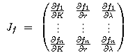
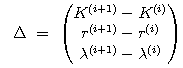
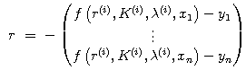
After that I used the Gauss-Newton algorithm to estimate the logistic function. The algorithm is given below.![]()
Then I used the LU decomposition of JfTJf and didn't accordingly find the inverse matrix of JfTJf to economize on computational resources. The example of the LU decomposition is given below.![]()
I also used the method of forward substitution to find b and the method of back substitution to find Δ.![]()
![]()
The convergence of r, K, and λ to the theoretical value is given below.
source code: GaussNewton.java
import java.awt.*;
import java.awt.event.*;
import java.text.DecimalFormat;
import java.applet.Applet;
import javax.swing.JLabel;
import javax.swing.JTextField;

public class GaussNewton extends Applet implements ActionListener{

	// variable set
	private static final long serialVersionUID = -1173026208646241820L;
	public static double r = 1.0;
	public static double k = 1.0;
	public static double c = 1.0;
	public static double[] s1 = new double[1000];
	public static double[] s2 = new double[1000];
	public static double[] s3 = new double[1000];
	public static double[] se1 = new double[1000];
	public static double[] k0 = new double[1000];
	public static double[] r0 = new double[1000];
	public static double[] c0 = new double[1000];
	public static double[] dk = new double[1000];
	public static double[] dr = new double[1000];
	public static double[] dc = new double[1000];
	public static double[] k3 = new double [3];
	public static double[] k4 = new double [3];
	public static double[] r3 = new double [3];
	public static int[] xxxx = new int [1000];
	public static int[] yyyy = new int [1000];
	public static int[] xxxx1 = new int [1000];
	public static int[] yyyy1 = new int [1000];
	public static double[][] Matrix = new double[3][3];
	public static double[][] MatrixL = new double[3][3];
	public static double[][] MatrixU = new double[3][3];
	public static double[][] MatrixU1 = new double[3][3];
	JTextField yx = new JTextField("1.0");
	JTextField yn = new JTextField("1.0");
	JTextField yr = new JTextField("1.0");
	JLabel label1 = new JLabel("The Example of The Gauss-Newton algorithm",JLabel.CENTER);
	JLabel label2 = new JLabel("<html><body><font size=3>The Growth Rate (0<r≤10<sup>8</sup>)</font></body></html>",JLabel.CENTER);
	JLabel label3 = new JLabel("<html><body><font size=3>The Carrying Capacity (0<K≤10<sup>8</sup>)</font></body></html>",JLabel.CENTER);
	JLabel label4 = new JLabel("<html><body><font size=3>The Integration Constant (-10<sup>8</sup><λ≤10<sup>8</sup>)</font></body></html>", JLabel.CENTER);

	public void init(){
		label1.setPreferredSize(new Dimension(416,24));
		label1.setFont(new Font("Serif",Font.BOLD,14));
		add(label1);
		label2.setPreferredSize(new Dimension(260,23));
		label2.setFont(new Font("Serif",Font.BOLD,11));
		add(label2);
		yx.setPreferredSize(new Dimension(80,23));
		add(yx);
		label3.setPreferredSize(new Dimension(260,23));
		label3.setFont(new Font("Serif",Font.BOLD,11));
		add(label3);
		yn.setPreferredSize(new Dimension(80,23));
		add(yn);
		label4.setPreferredSize(new Dimension(260,23));
		label4.setFont(new Font("Serif",Font.BOLD,11));
		add(label4);
		yr.setPreferredSize(new Dimension(80,23));
		add(yr);
		yx.addActionListener(this);
		yn.addActionListener(this);
		yr.addActionListener(this);
	}

	public void actionPerformed(ActionEvent e){
		if(e.getSource()==yx){
			r=Double.valueOf(yx.getText()).doubleValue();
			if(r <= 0 || r > Math.pow(10.0,8)){
				r = 1.0;
			}
		}
		if(e.getSource()==yn){
			k = Double.valueOf(yn.getText()).doubleValue();
			if(k <= 0 || k > Math.pow(10.0,8)){
				k = 1.0;
			}
		}
		if(e.getSource()==yr){c = Double.valueOf(yr.getText())
		.doubleValue();
			if(c < -Math.pow(10.0,8) || c > Math.pow(10.0,8)){c = 1.0;}
		}
		yx.setText(""+r);
		yn.setText(""+k);
		yr.setText(""+c);
		repaint();
	}

	public void paint(Graphics g){

		s1[0] = (Math.log(Math.abs(c))+Math.log(k)-Math.log(999))/r;
		s1[999] = (Math.log(Math.abs(c))+Math.log(k)+Math.log(999))/r;
		double aa=(s1[999]-s1[0])/999;
		s2[0]=function(k,r,c,s1[0]);
		s2[999]=function(k,r,c,s1[999]);
		for(int i=1;i<999;i++){
			s1[i]=s1[i-1]+aa;
		}
		for(int i=1;i<999;i++){
			s2[i]=function(k,r,c,s1[i]);
		}
		for(int i=0;i<1000;i++){
			se1[i]=normal.sampleNormal(0,k/50);
		}
		for(int i=0;i<1000;i++){
			s3[i]=s2[i]+se1[i];
		}
		for(int i=0;i<3;i++){
			for(int j=0;j<3;j++){
				Matrix[i][j]=0;
			}
		}

		k0[0]=k;
		r0[0]=r;
		c0[0]=c;

		for(int h=0;h<999;h++){
			for(int i=0;i<1000;i++){
				dk[i] = (1+c0[h]*k0[h]*Math.exp(r0[h]*(-s1[i]))-k0[h]*c0[h]*Math.exp(r0[h]*(-s1[i])))/Math.pow(1+c0[h]*k0[h]*Math.exp(r0[h]*(-s1[i])),2);
				dr[i] = -Math.pow(k0[h],2)*(-s1[i])*c0[h]*Math.exp(r0[h]*(-s1[i]))/Math.pow(1+c0[h]*k0[h]*Math.exp(r0[h]*(-s1[i])),2);
				dc[i] = -Math.pow(k0[h],2)*Math.exp(r0[h]*(-s1[i]))/Math.pow(1+c0[h]*k0[h]*Math.exp(r0[h]*(-s1[i])),2);
				Matrix[0][0]=Matrix[0][0]+Math.pow(dk[i],2);
				Matrix[0][1]=Matrix[0][1]+dk[i]*dr[i];
				Matrix[0][2]=Matrix[0][2]+dk[i]*dc[i];
				Matrix[1][0]=Matrix[1][0]+dr[i]*dk[i];
				Matrix[1][1]=Matrix[1][1]+Math.pow(dr[i],2);
				Matrix[1][2]=Matrix[1][2]+dr[i]*dc[i];
				Matrix[2][0]=Matrix[2][0]+dc[i]*dk[i];
				Matrix[2][1]=Matrix[2][1]+dc[i]*dr[i];
				Matrix[2][2]=Matrix[2][2]+Math.pow(dc[i],2);
			}

			MatrixU[0][0]=Matrix[0][0];
			MatrixU[0][1]=Matrix[0][1];
			MatrixU[0][2]=Matrix[0][2];
			MatrixU[1][0]=0;
			MatrixU[1][1]=Matrix[1][1]-Matrix[0][1]*Matrix[1][0]/Matrix[0][0];
			MatrixU[1][2]=Matrix[1][2]-Matrix[0][2]*Matrix[1][0]/Matrix[0][0];
			MatrixU[2][0]=0;
			MatrixU[2][1]=Matrix[2][1]-Matrix[0][1]*Matrix[2][0]/Matrix[0][0];
			MatrixU[2][2]=Matrix[2][2]-Matrix[0][2]*Matrix[2][0]/Matrix[0][0];
			MatrixU1[2][0]=0;
			MatrixU1[2][1]=0;
			MatrixU1[2][2]=MatrixU[2][2]-MatrixU[1][2]*MatrixU[2][1]/MatrixU[1][1];
			MatrixL[0][0]=1;
			MatrixL[0][1]=0;
			MatrixL[0][2]=0;
			MatrixL[1][0]=Matrix[1][0]/Matrix[0][0];
			MatrixL[1][1]=1;
			MatrixL[1][2]=0;
			MatrixL[2][0]=Matrix[2][0]/Matrix[0][0];
			MatrixL[2][1]=MatrixU[2][1]/MatrixU[1][1];
			MatrixL[2][2]=1;

			r3[0]=0;
			r3[1]=0;
			r3[2]=0;

			for(int i=0;i<1000;i++){
				r3[0]=r3[0]-dk[i]*(k0[h]/(1+c0[h]*k0[h]*Math.exp(r0[h]*(-s1[i])))-s3[i]);
				r3[1]=r3[1]-dr[i]*(k0[h]/(1+c0[h]*k0[h]*Math.exp(r0[h]*(-s1[i])))-s3[i]);
				r3[2]=r3[2]-dc[i]*(k0[h]/(1+c0[h]*k0[h]*Math.exp(r0[h]*(-s1[i])))-s3[i]);
			}

			k4[0]=r3[0];
			k4[1]=r3[1]-MatrixL[1][0]*k4[0];
			k4[2]=r3[2]-MatrixL[2][0]*k4[0]-MatrixL[2][1]*k4[1];
			k3[2]=k4[2]/MatrixU1[2][2];
			k3[1]=(k4[1]-MatrixU[1][2]*k3[2])/MatrixU[1][1];
			k3[0]=(k4[0]-MatrixU[0][1]*k3[1]-MatrixU[0][2]*k3[2])/MatrixU[0][0];
			k0[h+1]=k0[h]+k3[0];
			r0[h+1]=r0[h]+k3[1];
			c0[h+1]=c0[h]+k3[2];
		}

		double	minss3 = s3[0];
		double	maxss3 = s3[0];

		if(c>=0){
			for(int i=0;i<1000;i++){
				if(s3[i]>maxss3){
					maxss3 = s3[i];
				}
			}
			for(int i=0;i<1000;i++){
				if(s3[i]<minss3){
					minss3 = s3[i];
				}
			}
		}
		if(c<0){
			for(int i=525;i<1000;i++){
				if(s3[i]>maxss3){
					maxss3 = s3[i];
				}
			}
			for(int i=0;i<475;i++){
				if(s3[i]<minss3){
					minss3 = s3[i];
				}
			}
		}
		for(int i=0;i<1000;i++){
			xxxx[i] = (int)(i*351/999)+33;
			yyyy[i] = 474-(int)((s3[i]-minss3)*351/(maxss3-minss3)*345/351+6);
		}
		for(int i=0;i<1000;i++){
			xxxx1[i] = (int)(i*351/999)+33;
			yyyy1[i] = 474-(int)((function(k0[999],r0[999],c0[999],s1[i])-minss3)*351/(maxss3-minss3)*345/351+6);
		}

		Graphics2D g2 = (Graphics2D)g;
		GradientPaint gp1 = new GradientPaint(0, 0, new Color(154,181,228), 0,470,new Color(225,232,245), true);
		g2.setPaint(gp1);
		g2.fillRect(0,0,416,503);
		super.paint(g);
		GradientPaint gp2 = new GradientPaint(0, 33, new Color(225,232,245), 0,351,new Color(154,181,228), true);
		g2.setPaint(gp2);
		g2.fillRect(33,123,354,351);
		GradientPaint gp4 = new GradientPaint(33, 227, new Color(192,88,77), 33,418,new Color(160,82,45), true);
		g2.setPaint(gp4);
		if(c>=0){
			for (int i=0;i<1000;i++){
 	 			g2.fillOval(xxxx[i], yyyy[i], 4, 4);
			}
		}
		if(c<0){
			for (int i=0;i<475;i++){
 	 			g2.fillOval(xxxx[i], yyyy[i], 4, 4);
			}
			for (int i=525;i<1000;i++){
	 			g2.fillOval(xxxx[i], yyyy[i], 4, 4);
			}
		}
		GradientPaint gp3 = new GradientPaint(33, 227, new Color(79,129,189), 33,418,new Color(65,105,225), true);
		g2.setPaint(gp3);
		BasicStroke BoldLine = new BasicStroke(2.8f);
		g2.setStroke(BoldLine);
		if(c>=0){
			for (int i=1;i<1000;i++){
				g2.drawLine(xxxx1[i-1], yyyy1[i-1], xxxx1[i], yyyy1[i]);
			}
		}
		if(c<0){
			for (int i=1;i<475;i++){
				g2.drawLine(xxxx1[i-1], yyyy1[i-1], xxxx1[i], yyyy1[i]);
			}
			for (int i=526;i<1000;i++){
  				g2.drawLine(xxxx1[i-1], yyyy1[i-1], xxxx1[i], yyyy1[i]);
			}
		}
		DecimalFormat df0 = new DecimalFormat("0.00");
		DecimalFormat df1 = new DecimalFormat("0.000");
		DecimalFormat df2 = new DecimalFormat("0.000000");
		for(int i=0;i<5;i++){
			g2.setFont(new Font ("Serif",Font.BOLD,12));
			g2.setColor (new Color(0,0,0));
			String subx = df1.format(s1[0+249*i]);
			g2.drawString(subx,14+88*i,488);
		}
		for(int i=1;i<5;i++){
			g2.setFont(new Font ("Serif",Font.BOLD,12));
			g2.setColor (new Color(0,0,0));
			String suby = df0.format(maxss3/4*i);
			g2.drawString(suby,3,484-87*i);
		}
		g2.setFont(new Font ("Serif",Font.BOLD,12));
		g2.setColor (new Color(0,0,0));
		g2.drawString("n = 1000",280,367);
		g2.drawString("r",280,387);
		g2.drawString("*",290,386);
		g2.drawString(" =",293,387);
		g2.drawString(df2.format(r0[999]),315,387);
		g2.drawString("k",280,407);
		g2.drawString("*",290,407);
		g2.drawString(" =",293,407);
		g2.drawString(df2.format(k0[999]),315,407);
		g2.drawString("c",280,427);
		g2.drawString("*",290,427);
		g2.drawString(" =",293,427);
		g2.drawString(df2.format(c0[999]),315,427);
		g2.drawString("y",15,115);
		g2.drawString("x",340,488);
	}

	public static double function(double k,double r,double c,
	double x){
		return k/(1+c*k*Math.exp(r*(-x)));
	}
}
source code: normal.java
import java.util.*;

public class normal {
    private static Random rnd = new Random(Calendar.getInstance().getTimeInMillis()+Thread.currentThread().getId());
    private static double u;
    public static double sampleNormal(double e0, double e1) {
        double e2;
        e2=Math.pow(e1,(0.5));
        u=e2*rnd.nextGaussian()+e0;
        return u;
    }
}
In conclusion the estimates of the parameters was susceptible to influences of the initial values of the
parameters under the Gauss-Newton algorithm. r and K could converge on the theoretical values when the initial values of the parameters was set to half of the theoretical values but λ couldn't converge under the same condition where a number of times of iteration was between 1000 and 10000. The form of f(xi) was the normal logistic curve when the value of λ was positive and the different curve when the value of λ was negative.
Finally I am happy to assist you in coding and
estimating the logistic function with the Gauss-
Newton algorithm in JAVA.

コメントする